Key Points to remember :
- Population referes to the whole group of apparently identical parts or components which are under consideration of statistical analysis.
- Sample is the small portion of the population that is randomly selected from the population for evaluation purpose.
- Variable refers to the characteristic under consideration of each part or component.
- Measure of Central tendency : A central tendany is the value which represents the most of the components in a sample. For example Mean or average is a measure of central tendency, similerly mode or median are also measures of central tendency. Mean gives us idea about the value that a characteristic has for most of the components. But there is one limitation in just measure of central tendency that it does not give idea about the spread of the characteristic from central value. Two samples may have same mean even though one has most values very close to the mean and another sample has most values at considerable distance from the mean. Here comes the concept of Deviation, which gives the idea about distance from the mean value.
- Standard deviation : It is defined as the root mean square deviation from the mean value.
- Variance is the square of the S.D.
- Coefficient of variance is defined as th ratio of the standard deviation to the arithmetic mean, generally multiplied by 100.
- Normal distribution is a method of probability distribution in which the data from samples is converted into SNV (Standard normal variate) and then form the graph values of SNV curve various probabilities or limits are determined. The SNV curve is symmetrical about mean.
Theory Questions and Answers
Q:1.What are the basic Cause of variations in dimensions and characteristics?What are the types of causes for variations?
Ans :it is practically impossible to produce large quantity of identical components which have exactly same geometrical and functional properties. The variations in aparently identical components are due to following reasons
1. variation in properties of materials
2. variation in manufacturing process
3. variation in workmanship
4. variation in manufacturing environment
Classification of Causes of variations
following are the two categories of causes of variations
1. Assignable causes : this causes do not occur at random, but are the result of change in material properties, manufacturing process, workmanship are the effect of environmental parameters. The assignable causes may be attributed to something, hands their name assignable causes.
2. Chance causes : this causes orca at random and cannot be assigned to a particular variable. these are due to complex or unknown parameters which can neither be measured on traced. they are natural to process and even though all conditions have been held at their best.
The focus of statistical consideration is on assignable causes.
Q:2.What do you mean by dispersion, how dispersion is measured?
Ans : Dispersion is nothin but the spread of the data about its mean value. Dispersion is defined as the spread of the observation is a population which shows the extent to which the observations are scattered.
The dispersion is measured by following parameters,
1) Range and Coefficient of range
2) Mean deviation
3) Standard deviation
4) Quartile deviation
1) Range and coefficient of range : Range is defined as the difference between two extreme values. Coefficient of range is the ratio of range to sum of extreme values. Range gives rough idea about the spread of the population, but it does not gives idea about the percentage of spread from mean.
2) Mean deviation : In simple words Deviation means how far from normal. Deviation is the absolute difference between an observation and its mean value, mean deviation is the average of all such distributions. This has also limitation that it may give the same mean even when the differences are spread more. So the Standard deviation comes into picture where we square the deviation.
3) Standard Deviation : It is defined as the root mean square deviation from the mean value. The precise difference between mean and standard deviation is that here we square the difference, so that the values which are more far from mean get proper reflection in the final outcome.
HERE IS THE ILLUSTRATION THAT WHY IT IS NECESSARY TO SQUARE THE DIFFERENCES
Let us consider that there are four values which are at a distance of +4,+4,-4,-4 from the mean value
Now If we just sum up the differences from the mean,the negatives cancel the positives:
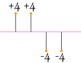 |
(4 + 4 − 4 − 4)/4 = 0 |
It simply doesnt work, here comes the idea of absolute values(ignoring sign)?
|
(|4| + |4| + |−4| + |−4|)/4 = (4 + 4 + 4 + 4)/4 = 4 |
That looks great, and that is what we do in Mean deviation, but here is one limitaion of Mean deviation:
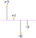 |
(|7| + |1| + |−6| + |−2|)/4 =( 7 + 1 + 6 + 2)/4 = 4 |
Following population also gives mean deviation as 4. Although the values are far away from mean tha above case.
So let us try squaring each difference (and taking the square root at the end):
|
√(42 + 42 + 42 + 42)/4 = √(64/4) = 4 | |
|
√(72 + 12 + 62 + 22)/4 = √(90)/4 = 4.74... |
That is perfect, The standard deviation is bigger when the differences are bigger..
This is why the standard deviation is most widely used to measure and represent dispersion of the population.
Following are the problems on Design of belt conveyor system collected from different university exams.
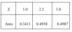
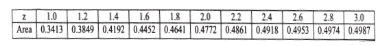
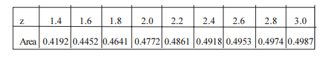
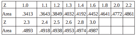
1)It is observed from a sample of 500 components that their  lengths are normally distributed with mean of 250.12 mm and standard deviation of 0.1mm. If the tolerances  specified by designer are 250 ± 0.15, find out the percentage of forgings rejected. Refer Table No: 01 for the Areas under normal distribution curve from Z = 0 to Z
Table No: 01 {Table is given at the end of this page}
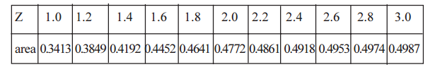
Shaft and hole assembly has following dimensions: Find what percentage of assemblies with clearance less than 0.15mm Refer Table No: 01 for the Areas under normal distribution curve from Z = 0 to Z {Table is given at the end of this page}
3)The diameters of bolts are normally distributed with a mean of 10.02mm and a standard deviation of 0.01 mm. The design specifications for the diameter are 10 ± 0.025 mm. Calculate the percentage of bolts which are likely to be rejected with given constrain. (The area below normal curve from Z = 0 to Z = 0.5 is 0.1915).
4) A mechanical component is subjected to a mean stress of 207 Mpa{Mega Pascal} with SD (Standard Deviation) of 55.2 Mpa. The material has a mean strength of 276 MPa with a SD(Standard deviation) of 41.4 MPa.
a) Find the probability of failure.
b) If the material is changed such that its mean strength is 380 MPa find the probability of failure.  Area from 0 to Z is as
5)The recommended class for fit between the recess and the spigot of rigid coupling is 60H6-j5. The dimensions of the two components is normally distributed and the specified tolerance is equal to the normal tolerance. Find the probability of interference fit between the two components. The tolerance is in microns and as follows :Area under SNV curve are from zero to z value are
6) A batch of spindles, to be used in machine tool, are designed for a meantorque transmitting capacity of 15N-m. The spindles are subjected to mean load torque of 10N-m. The torque transmitting capacity as well as the load torque are normally distributed with a standard deviation of 2N-m and 2.5N-m respectively. Estimate the percentage of spindles likely to fail. The areas under the standard normal distribution curve from zero to Z are follows:
7) A particular type of rolling contact bearing has a normally distributed time to failure, with a mean of 10,000 hrs and a standard deviation of 750h. If there are 100 such bearings fitted at a time, how many may be expected to ail within the first 11000 h? (Area below normal curve from Z = 0 to Z = 1.35 is given below)
8)A metal shaft of yield strength 180 MPa has a mean stress of 140 MPa. How many shafts will fail if the stresses and the yield strength are normally distributed with standard deviation of 20 MPa? Draw neat figures and use Area under the standard normal distribution curve from 0 to Z as,

9)It is observed from a sample of 1000 bearings bushes that the internal diameters are normally distributed with mean of 50.015 mm and standard deviation of 0.008mm. Dimension of this diameter specified on drawing is 50.01+0.1mm. Calculate the approximate number of rejected bushes from that sample. Refer Table No : 03 for the Areas under normal distribution curve from Z = 0 to Z
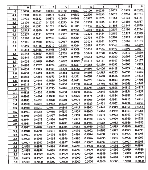
10) It is observed from a sample of 300 forgings that the lengths are normally distributed with mean of 150.5 mm and standard deviation of 0.02mm. Determine the tolerances specified by designer if 15 jobs are rejected. Refer Table No: 02 for the Areas under normal distribution curve from Z = 0 to Z ,Table No : 02
z |
0 |
1 |
2 |
3 |
4 |
5 |
6 |
7 |
8 |
9 |
0.0 |
0.0000 |
0.0040 |
0.0080 |
0.0120 |
0.0160 |
0.0199 |
0.0239 |
0.0279 |
0.0319 |
0.0359 |
0.1 |
0.0398 |
0.0438 |
0.0478 |
0.0517 |
0.0557 |
0.0596 |
0.0636 |
0.0675 |
0.0714 |
0.0754 |
0.2 |
0.0793 |
0.0832 |
0.0871 |
0.0910 |
0.0948 |
0.0987 |
0.1026 |
0.1064 |
0.1103 |
0.1141 |
0.3 |
0.1179 |
0.1217 |
0.1255 |
0.1293 |
0.1331 |
0.1368 |
0.1406 |
0.1443 |
0.1480 |
0.1517 |
0.4 |
0.1554 |
0.1591 |
0.1628 |
0.1664 |
0.1700 |
0.1736 |
0.1772 |
0.1808 |
0.1844 |
0.1879 |
0.5 |
0.1915 |
0.1950 |
0.1985 |
0.2019 |
0.2054 |
0.2088 |
0.2123 |
0.2157 |
0.2190 |
0.2224 |
0.6 |
0.2258 |
0.2291 |
0.2324 |
0.2357 |
0.2389 |
0.2422 |
0.2454 |
0.2486 |
0.2518 |
0.2549 |
0.7 |
0.2580 |
0.2612 |
0.2642 |
0.2673 |
0.2704 |
0.2734 |
0.2764 |
0.2794 |
0.2823 |
0.2852 |
0.8 |
0.2881 |
0.2910 |
0.2939 |
0.2967 |
0.2996 |
0.3023 |
0.3051 |
0.3079 |
0.3106 |
0.3133 |
0.9 |
0.3159 |
0.3186 |
0.3212 |
0.3238 |
0.3264 |
0.3289 |
0.3315 |
0.3340 |
0.3365 |
0.3389 |
1.0 |
0.3413 |
0.3438 |
0.3461 |
0.3485 |
0.3508 |
0.3531 |
0.3554 |
0.3577 |
0.3599 |
0.3621 |
1.1 |
0.3643 |
0.3665 |
0.3686 |
0.3708 |
0.3729 |
0.3749 |
0.3770 |
0.3790 |
0.3810 |
0.3830 |
1.2 |
0.3849 |
0.3869 |
0.3888 |
0.3907 |
0.3925 |
0.3944 |
0.3962 |
0.3980 |
0.3997 |
0.4015 |
1.3 |
0.4032 |
0.4049 |
0.4066 |
0.4082 |
0.4099 |
0.4115 |
0.4131 |
0.4147 |
0.4162 |
0.4177 |
1.4 |
0.4192 |
0.4207 |
0.4222 |
0.4236 |
0.4251 |
0.4265 |
0.4279 |
0.4292 |
0.4306 |
0.4319 |
1.5 |
0.4332 |
0.4345 |
0.4357 |
0.4370 |
0.4382 |
0.4394 |
0.4406 |
0.4418 |
0.4430 |
0.4441 |
1.6 |
0.4452 |
0.4463 |
0.4474 |
0.4485 |
0.4495 |
0.4505 |
0.4515 |
0.4525 |
0.4535 |
0.4545 |
1.7 |
0.4554 |
0.4564 |
0.4573 |
0.4582 |
0.4591 |
0.4599 |
0.4608 |
0.4616 |
0.4625 |
0.4633 |
1.8 |
0.4641 |
0.4649 |
0.4656 |
0.4664 |
0.4671 |
0.4678 |
0.4686 |
0.4693 |
0.4700 |
0.4706 |
1.9 |
0.4713 |
0.4719 |
0.4726 |
0.4732 |
0.4738 |
0.4744 |
0.4750 |
0.4756 |
0.4762 |
0.4767 |
2.0 |
0.4773 |
0.4778 |
0.4783 |
0.4788 |
0.4793 |
0.4798 |
0.4803 |
0.4808 |
0.4812 |
0.4817 |
2.1 |
0.4821 |
0.4826 |
0.4830 |
0.4834 |
0.4838 |
0.4842 |
0.4846 |
0.4850 |
0.4854 |
0.4857 |
2.2 |
0.4861 |
0.4865 |
0.4868 |
0.4871 |
0.4875 |
0.4878 |
0.4881 |
0.4884 |
0.4887 |
0.4890 |
2.3 |
0.4893 |
0.4896 |
0.4898 |
0.4901 |
0.4904 |
0.4906 |
0.4909 |
0.4911 |
0.4913 |
0.4916 |
2.4 |
0.4918 |
0.4920 |
0.4922 |
0.4925 |
0.4927 |
0.4929 |
0.4931 |
0.4932 |
0.4934 |
0.4936 |
2.5 |
0.4938 |
0.4940 |
0.4941 |
0.4943 |
0.4945 |
0.4946 |
0.4948 |
0.4949 |
0.4951 |
0.4952 |
2.6 |
0.4953 |
0.4955 |
0.4956 |
0.4957 |
0.4959 |
0.4960 |
0.4961 |
0.4962 |
0.4963 |
0.4964 |
2.7 |
0.4965 |
0.4966 |
0.4967 |
0.4968 |
0.4969 |
0.4970 |
0.4971 |
0.4972 |
0.4973 |
0.4974 |
2.8 |
0.4974 |
0.4975 |
0.4976 |
0.4977 |
0.4977 |
0.4978 |
0.4979 |
0.4980 |
0.4980 |
0.4981 |
2.9 |
0.4981 |
0.4982 |
0.4983 |
0.4983 |
0.4984 |
0.4984 |
0.4985 |
0.4985 |
0.4986 |
0.4986 |
3.0 |
0.4987 |
0.4987 |
0.4987 |
0.4988 |
0.4988 |
0.4989 |
0.4989 |
0.4989 |
0.4990 |
0.4990 |
3.1 |
0.4990 |
0.4991 |
0.4991 |
0.4991 |
0.4992 |
0.4992 |
0.4992 |
0.4992 |
0.4993 |
0.4993 |
3.2 |
0.4993 |
0.4993 |
0.4994 |
0.4994 |
0.4994 |
0.4994 |
0.4994 |
0.4995 |
0.4995 |
0.4995 |
3.3 |
0.4995 |
0.4995 |
0.4996 |
0.4996 |
0.4996 |
0.4996 |
0.4996 |
0.4996 |
0.4996 |
0.4997 |
3.4 |
0.4997 |
0.4997 |
0.4997 |
0.4997 |
0.4997 |
0.4997 |
0.4997 |
0.4997 |
0.4998 |
0.4998 |
3.5 |
0.4998 |
0.4998 |
0.4998 |
0.4998 |
0.4998 |
0.4998 |
0.4998 |
0.4998 |
0.4998 |
0.4998 |
3.6 |
0.4998 |
0.4999 |
0.4999 |
0.4999 |
0.4999 |
0.4999 |
0.4999 |
0.4999 |
0.4999 |
0.4999 |
3.7 |
0.4999 |
0.4999 |
0.4999 |
0.4999 |
0.4999 |
0.4999 |
0.4999 |
0.4999 |
0.4999 |
0.4999 |
3.8 |
0.4999 |
0.4999 |
0.4999 |
0.4999 |
0.4999 |
0.4999 |
0.4999 |
0.5000 |
0.5000 |
0.5000 |
3.9 |
0.5000 |
0.5000 |
0.5000 |
0.5000 |
0.5000 |
0.5000 |
0.5000 |
0.5000 |
0.5000 |
0.5000 |
4.0 |
0.5000 |
0.5000 |
0.5000 |
0.5000 |
0.5000 |
0.5000 |
0.5000 |
0.5000 |
0.5000 |
0.5000 |
11)A rigid coupling is assembled with recommended fit 60 H6-j5 between the recess and the spigot. The dimensions of the two components are normally distributed and the specified tolerance is equal to the natural tolerance. Determine the probability of interference fit between the two components.The tolerances in micron are as follows:The area under standard normal variate curve are as follows,
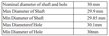
12)A shaft and hole assembly of nominal diameter 40 mm have following dimensions. Hole- Max diameter 40.1 mm; Minimum diameter 40.0 mm; Shaft- Max diameter 39.9mm ; Minimum diameter 39.85 mm. Assuming the shaft and hole dimensions are normally distributed determine; [12] i) the % of assemblies having clearance less than 0.15 mm ; and ii) the % of assemblies having clearance greater than 0.22 mm The areas under the standard normal distribution curve from zero to Z are as follows;
- Log in to post comments